Online Campaign Performance

Marketing Analysis

Code

library(bigrquery)
library(tidyverse)
library(highcharter)
library(plotly)
library(lubridate)
library(echarts4r)
library(broom)
library(flextable)
library(reactable)
library(GGally)
library(jtools)
library(ggstatsplot)
library(viridis)
library(ggpubr)
library(htmltools)
library(ggpubr)

# library(dlookr)


# avoid the conflict with MASS::select
select <- dplyr::select

# local folder
# "~/Dropbox/turing_college/Modules/Marketing_Analysis/"

Assignment

Data from the google merchandise store contains information about every browsing event from the user (e.g. page view, click item, scroll), as well as its date, timestamp, order amount and other device-specific information.

Currently we are interested in analyzing the outcome of our marketing campaigns in the period from November 2020 to the end of January 2021.

In particular, we are interested in assessing:

• whether the campaigns resulted in a higher conversion from browsing to purchasing
• whether this is related to the amount of time spent on the website (session length)
• what was the impact on the revenues

Importantly, we are also interested to carry out the analysis for each day of the week to assess whether there are some noticeable seasonal patterns.

Data Preparation

Code

# The data was too big to be exported in one csv, so we have to download
# individual months and row-bind them

nov <- read_csv("01_nov.csv")
dec <- read_csv("02_dec.csv")
jan <- read_csv("03_jan.csv")

df <- rbind(nov, dec, jan) 

df <- df %>% 
 
 # rename session_length as TTP (Time-To-Purchasing) and threshold to 1 hour
 rename(TTP = session_length) %>% 
 filter(TTP > 300, TTP < 3600) %>% 

 # mutate(campaign = ifelse(campaign == "(data deleted)", "generic_campaign", campaign)) %>% 
 # mutate(campaign = factor(campaign)) %>% 
 
 # identify sessions with purchase and browse-only sessions
 mutate(revenue = ifelse(is.na(revenue), 0, revenue)) %>% 
 mutate(purchase_session = ifelse(revenue > 0, "YES", "NO") %>% factor) %>% 
  
 # create columns for weekday_name and weekday_number
 mutate(weekday_num = wday(event_date, week_start = 1) %>% factor) %>% 
 mutate(weekday_name = wday(event_date, week_start = 1, label = T) %>% factor) 

Identifying sessions

The database does not contain unequivocal information about the start and the end of a session, therefore we had to devise a suitable procedure for the existing data. This was carried out in SQL (the dataset consists of ~4 million rows). In brief:

• The session_start event was chosen to define the start of the session. Within the same day, different events with event_name="session_start" were assigned a rank according to their timestamp
• Every other event before the next session_start was labelled with this rank
• Session length was calculated as the difference in seconds between the session_start event and the last event before the subsequent session_start
• Events with no rank are those which belong to sessions started the day before, and were therefore not further considered

Thresholding session length

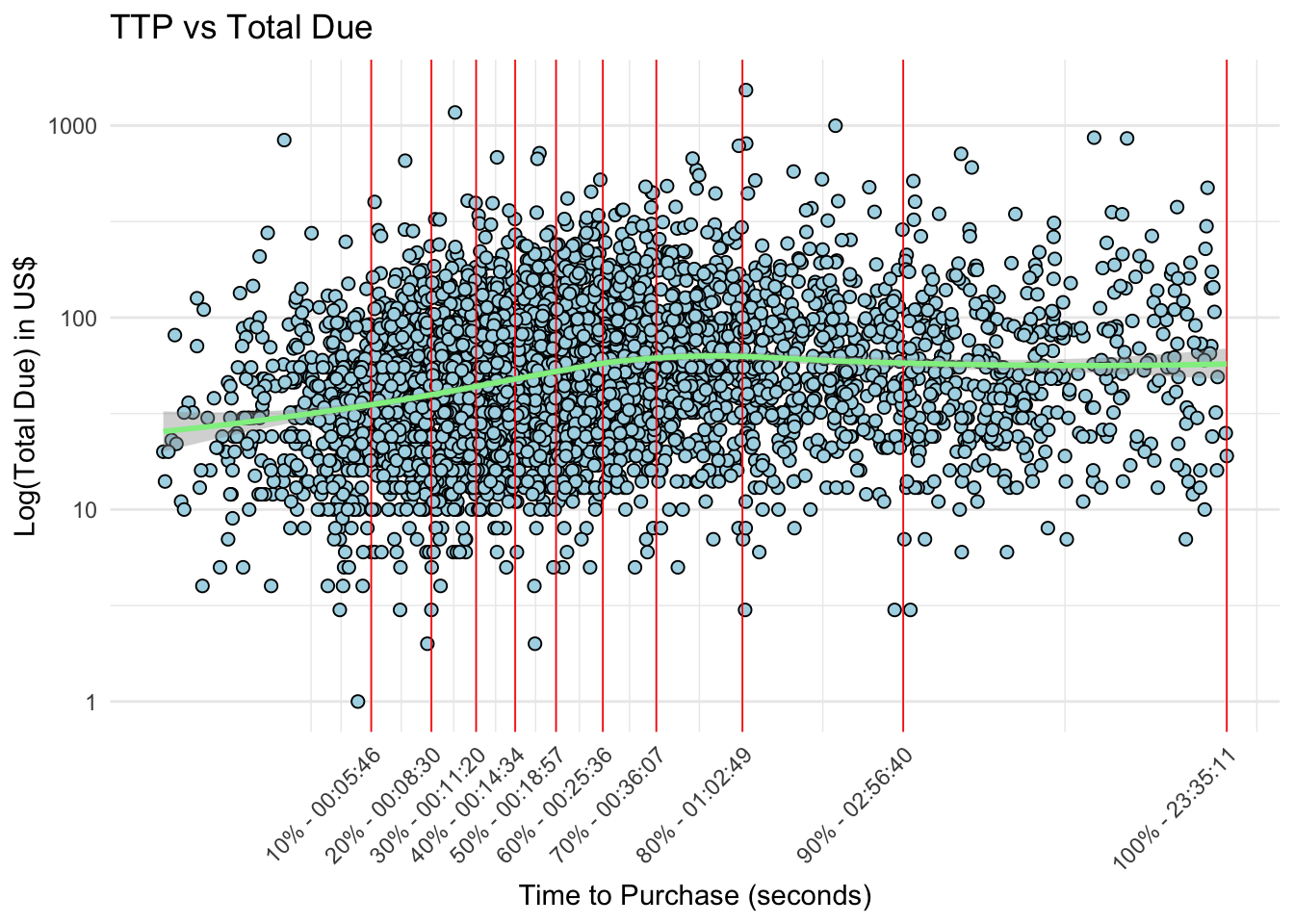
In a previous Product Analysis we observed that the median length of a session is ~ 20 minutes, and that the order amount stops increasing for sessions longer than 30-60 minutes.

Therefore we chose to focus on session no longer than 3600 seconds (1 hour). We also repeated the analyses below with other thresholds (20, 120 minutes or no threshold) and we observed virtually identical results.

Pooling all campaigns together

We know that there is a problem with the data: the campaign reference of the purchases (e.g. Black Friday or New Year’s eve) are lost, and were replaced with (data_deleted). The very few remaining are related to events in sessions where the campaign was not recorded in the purchase event row, but still present among the events of that session - therefore we decided to assign that purchase to that campaign.

Still, the number of purchases in different campaigns is negligible with respect to the total number of data points, which prevents us to stratify the analysis per campaign.

Code

df %>% 
 select(campaign, purchase_session) %>% 
 group_by(campaign, purchase_session) %>% 
 count %>% 
 mutate(
  purchase_session = ifelse(purchase_session=="YES","purchase session","browsing only")
 ) %>% 
 pivot_wider(names_from = purchase_session, values_from = n) %>% 
 mutate(`purchase session` = ifelse(is.na(`purchase session`),0,`purchase session`)) %>% 
 flextable

campaign	browsing only	purchase session
(data deleted)	848	62
BlackFriday_V1	1	0
BlackFriday_V2	1	0
Data Share Promo	152	0
Holiday_V2	1	0
NewYear_V1	4	0
NewYear_V2	2	0
none	50,799	3,822

Therefore we will aggregate all the different campaigns into a generic campaign YES/NO column, and examine the other metrics (revenue and TTP) according to whether they relate to any campaign or to no campaign.

Code

df <- df %>% 
 mutate(campaign = ifelse(campaign == "none", "NO", "YES") %>% factor)

Analysis

Fail to increase conversion rate

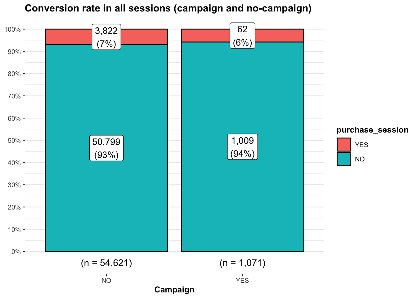
Overall, we don’t obseve a difference in the conversion rate - from browsing only to purchasing - due to campains

When no campaigns are present on the website, 7% of all the visits result in a purchase. Comparably, when a campaign is running, 6% of the visitors end up purchasing.

The conversion rate for campaign sessions appears to be slightly higher on Thursday and Friday, but not more than what can be expected by chance.

Overall conversion rate

Code

contingency_table <- df %>% 
  select(campaign, purchase_session) %>% 
  group_by(campaign, purchase_session) %>% 
  count() %>% 
  pivot_wider(names_from = purchase_session, values_from = n, values_fill = 0)

# --------------  ggbarstats --------------------------

# Conversion rate across all days
ggbarstats(
 data = df,
 x = purchase_session,
 y = campaign,
 label = "both",
 results.subtitle = F
) + 
 scale_fill_manual(values = c("#F8766D","#00BFC4")) +
 labs(
  title = "Conversion rate in all sessions (campaign and no-campaign)",
  x = "Campaign"
 )

Code

# The following two are replaced by the line plot in the next tab

# # Conversion rate for each day in campaign sessions
# ggbarstats(
#  data = df %>% filter(campaign == "YES"),
#  x = purchase_session,
#  y = weekday_name,
#  label = "both",
#  results.subtitle = F
# ) +
#  scale_fill_manual(values = c("#F8766D","#00BFC4")) +
#  labs(
#   title = "Conversion rate in campaign sessions",
#   x = "Day of the week"
#  )
# 
# 
# 
# # Conversion rate for each day in no-campaign sessions
# ggbarstats(
#  data = df %>% filter(campaign == "NO"),
#  x = purchase_session,
#  y = weekday_name,
#  label = "both",
#  results.subtitle = F
# ) +
#  scale_fill_manual(values = c("#F8766D","#00BFC4")) +
#  labs(
#   title = "Conversion rate in NO-campaign sessions",
#   x = "Day of the week"
#  )

Per weekday

Code

# Barplot and line plot of the conversion rates
ddf <- df %>%
 group_by(weekday_name, campaign, purchase_session) %>% 
 count() %>% 
 group_by(weekday_name, campaign) %>% 
 mutate(total = sum(n)) %>% 
 filter(purchase_session == "YES") %>% 
 mutate(conversion_rate = round(n/total*100,1))  
 # select(weekday_name, campaign, conversion_rate)


ddf %>%
 mutate(campaign = fct_rev(campaign)) %>% 
 ggplot(
  aes(x = weekday_name, y = conversion_rate, color = campaign, 
      group = campaign,
      text = paste("Campaign:", campaign, "<br>Conversion Rate:", conversion_rate, "%"))
 ) +
 # geom_bar(aes(fill = campaign), stat = "identity", position = "dodge") +
 geom_line() +
 geom_point() +
 theme_minimal() +
 labs(
  title = "Conversion rate for campaing and no-campaign sessions",
  x = "Day of the week",
  y = "Conversion Rate"
 ) +
 scale_y_continuous(labels = scales::percent_format(scale = 1)) -> gg

ggplotly(gg, tooltip = "text", config = list(displayModeBar = FALSE))

No significant difference in proportions

Code

# Wednesday
prop_Thu <- ddf %>% 
 filter(weekday_name == "Wed") %>% 
 rename(n_converted = n) %>% 
 ungroup() %>% 
 select(n_converted, total) %>% 
 arrange(total)

cat("Wednesday")

Wednesday

Code

prop.test(x = prop_Thu$n_converted, n = prop_Thu$total, alternative = "greater")

    2-sample test for equality of proportions with continuity correction

data:  prop_Thu$n_converted out of prop_Thu$total
X-squared = 1.388e-28, df = 1, p-value = 0.5
alternative hypothesis: greater
95 percent confidence interval:
 -0.03071573  1.00000000
sample estimates:
    prop 1     prop 2 
0.07179487 0.07021663 

Code

# Thursday
prop_Thu <- ddf %>% 
 filter(weekday_name == "Thu") %>% 
 rename(n_converted = n) %>% 
 ungroup() %>% 
 select(n_converted, total) %>% 
 arrange(total)

cat("Thursday")

Thursday

Code

prop.test(x = prop_Thu$n_converted, n = prop_Thu$total, alternative = "greater")

    2-sample test for equality of proportions with continuity correction

data:  prop_Thu$n_converted out of prop_Thu$total
X-squared = 1.2833e-28, df = 1, p-value = 0.5
alternative hypothesis: greater
95 percent confidence interval:
 -0.02947896  1.00000000
sample estimates:
    prop 1     prop 2 
0.06349206 0.06127591 

Code

# Friday
prop_Fri <- ddf %>% 
 filter(weekday_name == "Fri") %>% 
 rename(n_converted = n) %>% 
 ungroup() %>% 
 select(n_converted, total) %>% 
 arrange(total)


cat("Friday")

Friday

Code

prop.test(x = prop_Fri$n_converted, n = prop_Fri$total, alternative = "greater")

    2-sample test for equality of proportions with continuity correction

data:  prop_Fri$n_converted out of prop_Fri$total
X-squared = 2.6122e-29, df = 1, p-value = 0.5
alternative hypothesis: greater
95 percent confidence interval:
 -0.03484194  1.00000000
sample estimates:
    prop 1     prop 2 
0.08187135 0.07921039 

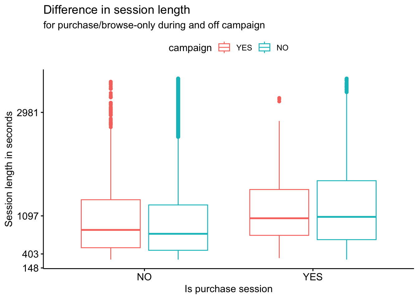
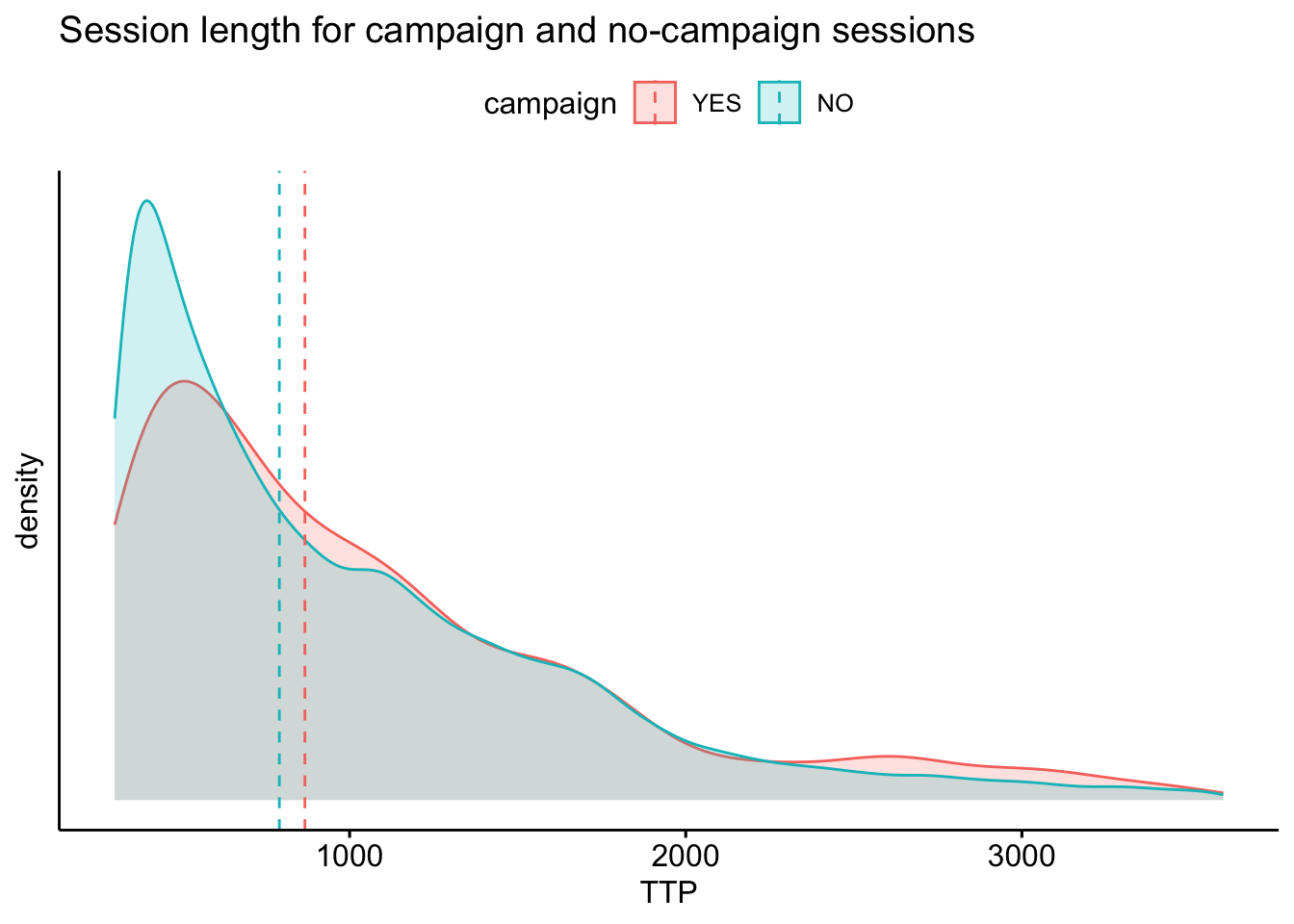
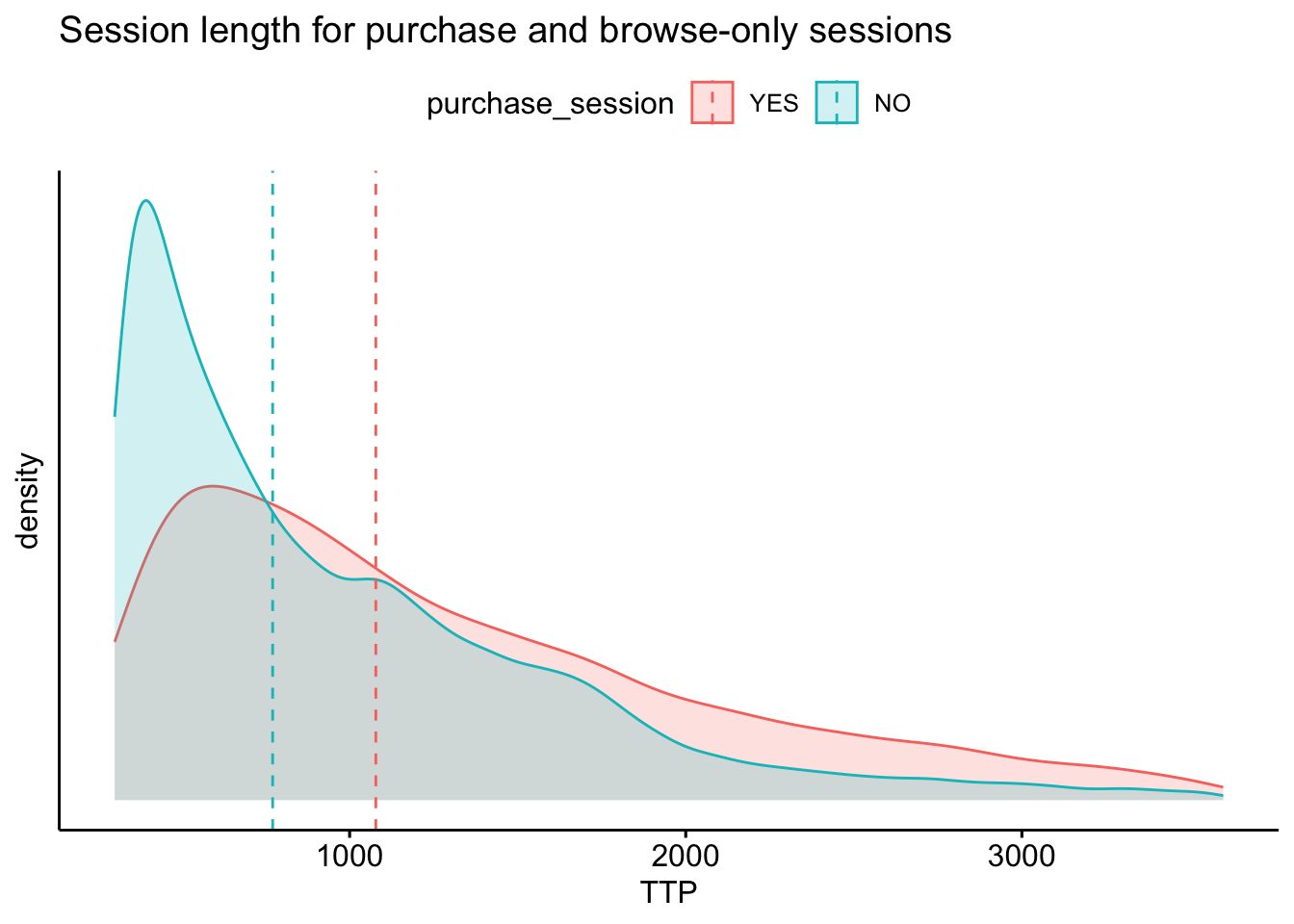
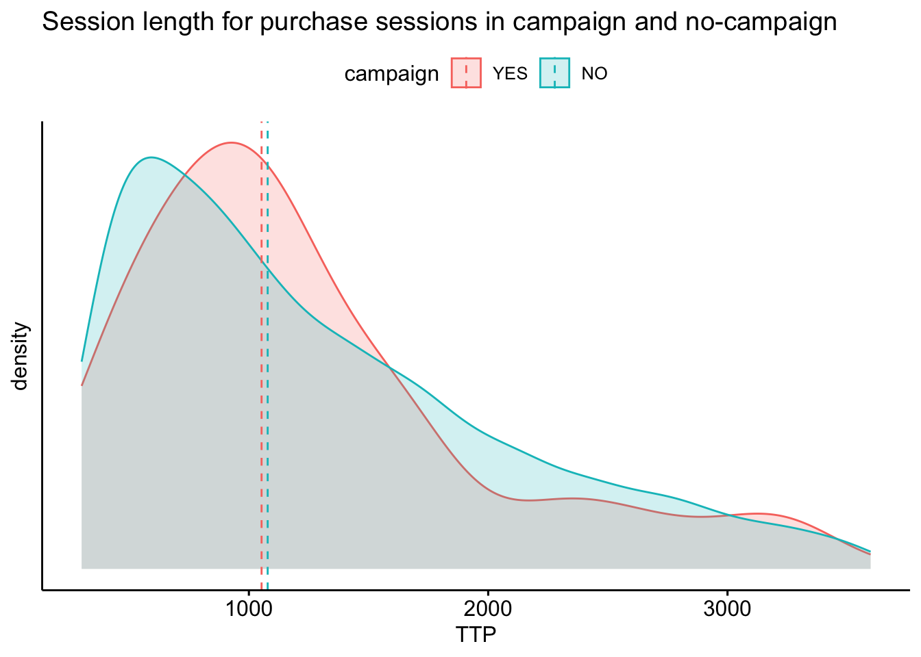
Session length differ, but not in an interesting way

Campaign sessions and purchase sessions (either on- or off-campaign) are significantly slighltly longer (up to 5 minutes) , however there is no interaction between campaign and session type (browse-only or purchasing). For instance, it is not the case that campaign sessions are longer for purchase and shorter for browse-only with respect to no-campaign sessions.

As expected from the previous anova, campaign sessions are slightly longer each day of the week, although the median value is associated with high variability.

On Saturday the purchasing campaign session is on average much shorter than the sessions not related to a campaign. However, a closer inspection shows that these are just 4 purchasing events, which makes a statistical comparison meaningless.

Session time by conversion and campaign

NB: Boxplots show session time in seconds, however anova2 was run on log(session_time) to approximate normally distributed values.

Code

ddf <- df %>% 
 select(TTP, campaign, purchase_session) %>%
 mutate(logTTP = log(TTP)) %>% 
 mutate(campaign = fct_rev(campaign))

# # Table
# ddf %>%
#  group_by(campaign, purchase_session) %>%
#  reframe(mean_TTP = mean(TTP))


ddf %>% 
 select(logTTP, campaign, purchase_session) %>% 
 ggboxplot(
  x = "purchase_session", y = "logTTP", color = "campaign"
 ) +
 scale_y_continuous(trans = "exp", labels = function(x)(round(exp(x)))) +
 labs(
  title = "Difference in session length",
  subtitle = "for purchase/browse-only during and off campaign",
  y = "Session length in seconds",
  x = "Is purchase session"
 )

Code

anova2 <- aov(formula = logTTP ~ campaign * purchase_session, data = ddf)
cat("Session time is higher for campaign and purchase, but there is no interaction")

Session time is higher for campaign and purchase, but there is no interaction

Code

summary(anova2)

                             Df Sum Sq Mean Sq F value   Pr(>F)    
campaign                      1      5    4.99  13.181 0.000283 ***
purchase_session              1    300  299.77 791.219  < 2e-16 ***
campaign:purchase_session     1      1    0.55   1.458 0.227199    
Residuals                 55688  21099    0.38                     
---
Signif. codes:  0 '***' 0.001 '**' 0.01 '*' 0.05 '.' 0.1 ' ' 1

Code

# plot(anova2)
# car::Anova(anova2, type = "III")

Session length during or outside a campaign

Code

# define a fn to produce the three following plots
plot_session_length <- function(df, title) {
 df %>% 
 group_by(weekday_name, campaign) %>% 
 reframe(
  weekday_name = unique(weekday_name),
  median_TTP = median(TTP),
  MAD_low = floor(median(TTP) - mad(TTP)),
  MAD_high = ceiling(median(TTP) + mad(TTP))
 ) %>%
 mutate(campaign = fct_rev(campaign)) %>%
 ggplot(aes(x = weekday_name, y = median_TTP, fill = campaign)) +
 geom_col(position = "dodge") +
 geom_errorbar(
  aes(ymin = MAD_low, ymax = MAD_high),
  position = position_dodge(width = 0.9),  # Adjust width for dodge position
  width = 0.2, color = "grey"  # Width of error bars
 ) +
 labs(title = title, 
      x = "Day of the week",
      y = "Median TTP") +
 theme_minimal() +
  theme(
    legend.position = "bottom",
    panel.grid.major.x = element_blank(),  # Remove vertical grid lines
    panel.grid.minor = element_blank()     # Remove minor grid lines
  ) -> gg

 return(ggplotly(gg) %>% config(displayModeBar = FALSE))
}


# overall session length (purchase and browse-only sessions)
plot_session_length(
 df,
 title = "Overall session length in- and outside campaign"
)

Session length for Purchasing sessions (TTP)

Code

plot_session_length(
 df %>% filter(purchase_session == "YES"),
 title = "Purchase sessions length in- and outside campaign"
)

Code

# # The following compares TTP for campaign and no-campaign
# # on Saturday, when the TTP appears shorter. However, a closer
# # inspection reveals that these are just 4 observations, therefore
# # a statistical test is meaningless

# ddf <- df %>%
#  filter(purchase_session == "YES", weekday_name == "Sat") %>%
#  select(campaign, TTP)
# 
# ggbetweenstats(
#  data = ddf,
#  x = campaign,
#  y = TTP
# ) + 
#  scale_y_continuous(trans = "log")
#
# ddf %>% filter(campaign == "YES")


# # The following carries out an anova TTP ~ weekday * campaign
# # There are no significant differences
# ddf <- df %>% 
#  filter(purchase_session == "YES") %>% 
#  select(TTP, campaign, weekday_name) %>% 
#  mutate(logTTP = log(TTP))
# 
# anova2 <- aov(TTP ~ campaign * weekday_name, data = ddf)
# summary(anova2)
# car::Anova(anova2, type = "III")

Browse-only sessions (no purchase)

Code

plot_session_length(
 df %>% filter(purchase_session == "NO"),
 title = "Browse-only sessions length in- and outside campaign"
)

Revenues highest at mid-week

The highest revenues for campaign-related orders were generated at mid-week, while they were much lower during the weekend and on Monday.

There are also differences in the median amount order between campaign and no-campaign sessions in some days, however not more than what could be expected by chance (assessed with an anova2).

Total revenue due to campaigns

Code

df %>%
  filter(purchase_session == "YES", campaign == "YES") %>%
  select(weekday_name, revenue) %>% 
  group_by(weekday_name) %>% 
  reframe(
    total_revenue = sum(revenue)
  ) %>% 
  ggplot(aes(x = weekday_name, y = total_revenue, 
   text = paste(weekday_name, "\n","Total Revenue: ", total_revenue, "US$"))
  ) +
  geom_bar(stat = "identity", fill = "#F8766D") +
  labs(
   title = "Total revenue from campaign orders",
   x = "Day of the week",
   y = "Total revenue in USD"
  ) +
  theme_minimal() -> gg

ggplotly(gg, tooltip = "text") %>% config(displayModeBar = FALSE)

Range of order values

Code

df %>%
 filter(purchase_session == "YES") %>%
 select(weekday_name, revenue, campaign) %>% 
 group_by(weekday_name, campaign) %>% 
 mutate(campaign = fct_rev(campaign)) %>%
 ggplot(aes(x = weekday_name, y = revenue, fill = campaign)) +
 geom_boxplot() +
 # scale_y_continuous(limits = c(0,120)) +
 scale_y_continuous(breaks = seq(0, max(df$revenue), by = 100)) +
 labs(
  title = "Order value in- and outside-campaign",
  x = "Day of the week",
  y = "Revenue"
 ) +
 theme_minimal() -> gg


ggplotly(gg) %>%
 layout(yaxis = list(range = c(0, 140))) %>% 
 layout(boxmode = "group")

Code

# Anova 2 : revenue ~ weekday_name * campaign
# No significant difference.

ddf <- df %>% 
 filter(purchase_session == "YES") %>% 
 select(revenue, weekday_name, campaign) %>% 
 mutate(log_revenue = log(revenue))

cat("No significant effect of of mean log_revenue or campaign")

No significant effect of of mean log_revenue or campaign

Code

anova2 <- aov(log_revenue ~ weekday_name * campaign, data = ddf)
summary(anova2)

                        Df Sum Sq Mean Sq F value Pr(>F)
weekday_name             6    4.5  0.7583   0.994  0.427
campaign                 1    0.0  0.0211   0.028  0.868
weekday_name:campaign    6    3.4  0.5662   0.742  0.615
Residuals             3870 2951.9  0.7628               

Code

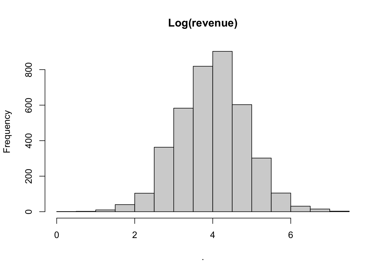
# Note that revenues are log-normally distributed
# however this has no effect on the anova2
df$revenue[df$revenue > 0] %>% log() %>% hist(main = "Log(revenue)")

Total revenues for in- and out-campaign

Code

df %>%
  filter(purchase_session == "YES") %>%
  select(weekday_name, revenue, campaign) %>% 
  group_by(weekday_name, campaign) %>% 
  mutate(campaign = fct_rev(campaign)) %>%
  reframe(
    total_revenue = sum(revenue)
  ) %>% 
  ggplot(aes(
   x = weekday_name, y = total_revenue, 
   fill = campaign, 
   text = paste(weekday_name, "\n","Total Revenue: ", total_revenue, "\n", "Campaign: ", campaign))
  ) +
  geom_bar(stat = "identity") +
  # scale_y_continuous(
  #   trans = "log",
  #   labels = function(x) round(x)
  # ) +
 theme_minimal() -> gg

ggplotly(gg, tooltip = "text")

ROI: 91.17%

Code

# NB: here we consider again the initial data, with no threshold for session duration

nov <- read_csv("01_nov.csv")
dec <- read_csv("02_dec.csv")
jan <- read_csv("03_jan.csv")

total_df <- rbind(nov, dec, jan)

marketing_cost <- read_csv("adsense_monthly.csv")
cost_of_campaigns <- sum(marketing_cost$Cost) %>% round(2)


campaigns_revenues <- total_df[total_df$campaign != "none", "revenue"] %>% na.omit() %>% sum

# campaigns_revenues <- total_df %>% 
#  filter(campaign != "none", !is.na(revenue)) %>%
#  select(revenue) %>% pull %>% sum


ROI <- campaigns_revenues / cost_of_campaigns

ROI_pct <- (round(ROI,4) - 1) * 100

KPI_name <- "Return on Investment"

Return on Investment: The total cost for marketing campaigns was 2432.45 US$. The revenues generated by these campaigns were 4650 US$.

Code

div(
  style = "display: flex; flex-wrap: wrap; justify-content: space-around; align-items: center; font-family: sans-serif;",
  div(
    style = "background-color: #f39c12; color: white; padding: 10px; border-radius: 5px; margin: 10px; text-align: center;",
    div(style = "font-size: 28px;", KPI_name),
    div(style = "font-size: 36px;", paste(ROI_pct, "%"))
  )
)

Return on Investment

91.17 %

Code

# table with the cost of every marketing campaign
marketing_cost %>% 
 group_by(Campaign) %>%
 reframe(
  cost = round(sum(Cost),2)
 ) %>% flextable()

Campaign	cost
BlackFriday_V1	164.49
BlackFriday_V2	364.14
Data Share Promo	1,430.17
Holiday_V1	143.78
Holiday_V2	129.10
NewYear_V1	44.30
NewYear_V2	156.47

Main takeaways

Overall, the campaigns did not appear to benefit revenues.

• The conversion rate was comparable between campaign and no-campaign sessions. Any apparent difference in specific days can be due to chance

• Campaigns slightly increased the total browsing time, but did not affect the session time in purchasing sessions overall and across weekdays

• Revenues from campaign were highest in mid-week days and lowes on weekends and on monday

• These results are comparable across different choices of session length

Appendix

Description

A few other potentially interesting plots which were used during the EDA for the presented analysis.

Revenues and orders per day on- and off-campaign

Code

# Daily number of orders

df %>% 
 filter(purchase_session == "YES") %>% 
 group_by(event_date, campaign) %>% 
 mutate(campaign = fct_rev(campaign)) %>%
 reframe(
  n_sales = n()
 ) %>% 
 ggplot(aes(x = event_date, y = n_sales, fill = campaign)) +
 # geom_area(position = "stack", alpha = 0.7) +  # Area
 geom_bar(stat = "identity", position = "stack", alpha = 0.7) +  # Bars
 # geom_line(aes(color = campaign), position = "stack") +  # Lines
 labs(
  title = "Number of sales per day",
  x = "Date", y = "Number of Orders"
 ) +
 theme_minimal() -> gg

ggplotly(gg)

Code

# Daily revenues

df %>% 
 filter(purchase_session == "YES") %>% 
 group_by(event_date, campaign) %>% 
 mutate(campaign = fct_rev(campaign)) %>%
 reframe(
  revenues = sum(revenue)
 ) %>% 
 ggplot(aes(x = event_date, y = revenues, fill = campaign)) +  
 geom_bar(stat = "identity", position = "stack", alpha = 0.7) +  # Bars
 # geom_area(position = "stack", alpha = 0.7) +  # Area
 labs(
  title = "Revenues per day",
  x = "Date", y = "Revenue in US$"
 ) +
 theme_minimal() -> gg

ggplotly(gg)

EDA of Session length

Code

df %>% 
 group_by(campaign) %>% 
 mutate(campaign = fct_rev(campaign)) %>%
 ggdensity(
  x = "TTP", add = "median", color = "campaign", fill = "campaign",
  alpha = 0.2, rug = F
 ) +
 labs(title = "Session length for campaign and no-campaign sessions") +
  theme(
   axis.ticks.y = element_blank(),   # Hide y-axis ticks
   axis.text.y = element_blank(),    # Hide y-axis labels
 )

Code

df %>% 
 group_by(purchase_session) %>% 
 mutate(purchase_session = fct_rev(purchase_session)) %>%
 ggdensity(
  x = "TTP", add = "median", color = "purchase_session", fill = "purchase_session",
  alpha = 0.2, rug = F
 ) +
 labs(title = "Session length for purchase and browse-only sessions") +
  theme(
   axis.ticks.y = element_blank(),   # Hide y-axis ticks
   axis.text.y = element_blank(),    # Hide y-axis labels
 )

Code

df %>% 
 group_by(campaign) %>% 
 filter(purchase_session == "YES") %>% 
 mutate(campaign = fct_rev(campaign)) %>%
 ggdensity(
  x = "TTP", add = "median", color = "campaign", fill = "campaign",
  alpha = 0.2, rug = F
 ) +
 labs(title = "Session length for purchase sessions in campaign and no-campaign") +
  theme(
   axis.ticks.y = element_blank(),   # Hide y-axis ticks
   axis.text.y = element_blank(),    # Hide y-axis labels
 )

Days in which the campaign was run

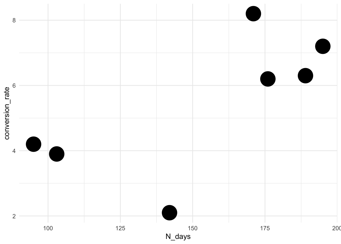
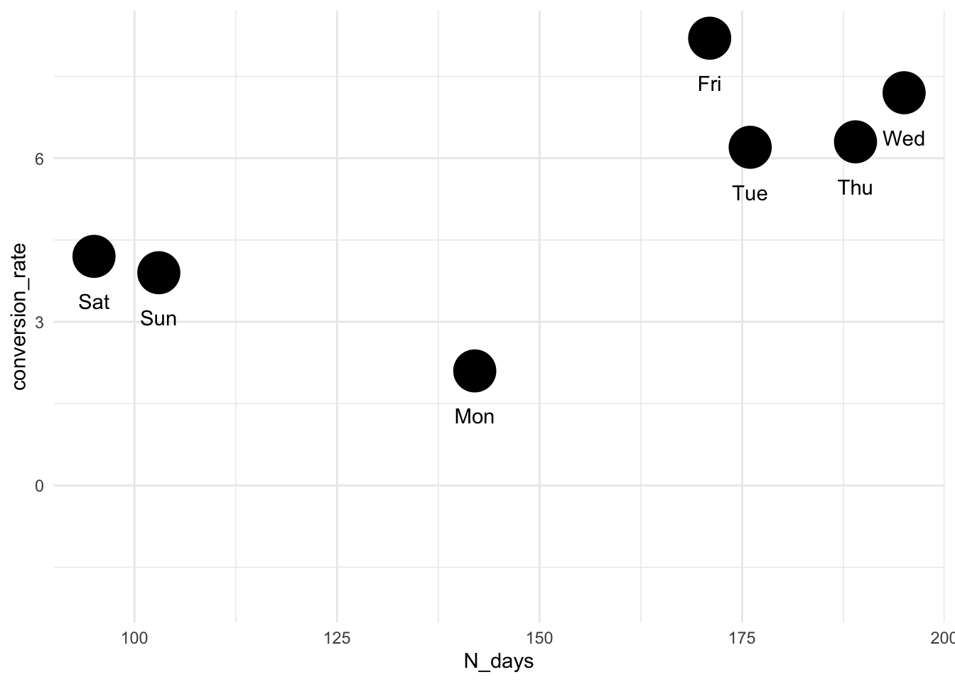
Could the differences in conversion rate and total revenue during campaign days be explained by substantial differences in the number of days in which the campaign was run?

Code

n_weekdays <- df %>% 
 group_by(weekday_name, campaign) %>% 
 count() %>% 
 pivot_wider(names_from = campaign, values_from = n) %>% 
 select(weekday_name, YES) %>% 
 rename(N_days = YES)



campaign_conversion_rates <- df %>%
 group_by(weekday_name, campaign, purchase_session) %>% 
 count() %>% 
 group_by(weekday_name, campaign) %>% 
 mutate(total = sum(n)) %>%
 ungroup %>% 
 filter(purchase_session == "YES", campaign == "YES") %>% 
 mutate(conversion_rate = round(n/total*100,1))  %>% 
 select(weekday_name, conversion_rate) 


n_weekdays %>% 
  inner_join(campaign_conversion_rates, by = "weekday_name") %>% 
 ggplot(aes(x = N_days, y = conversion_rate)) +
 geom_point(size=10) +
 theme_minimal()

Code

n_weekdays %>%
  inner_join(campaign_conversion_rates, by = "weekday_name") %>%
  ggplot(aes(x = N_days, y = conversion_rate, label = weekday_name)) +
  geom_point(size = 10) +
  geom_text(vjust = 3.5) +  # Adjust the vertical position of the labels
  ylim(-2, NA) +  # Set the y-axis limits to start from -2
  theme_minimal()